Methods for data scaling, transformation and normalisation.
Usage
transformArcSine(d)

# S4 method for AnalysisData
transformArcSine(d)

transformAuto(d)

# S4 method for AnalysisData
transformAuto(d)

transformCenter(d)

# S4 method for AnalysisData
transformCenter(d)

transformLevel(d)

# S4 method for AnalysisData
transformLevel(d)

transformLn(d, add = 1)

# S4 method for AnalysisData
transformLn(d, add = 1)

transformLog10(d, add = 1)

# S4 method for AnalysisData
transformLog10(d, add = 1)

transformPareto(d)

# S4 method for AnalysisData
transformPareto(d)

transformPercent(d)

# S4 method for AnalysisData
transformPercent(d)

transformRange(d)

# S4 method for AnalysisData
transformRange(d)

transformSQRT(d)

# S4 method for AnalysisData
transformSQRT(d)

transformTICnorm(d, refactor = TRUE)

# S4 method for AnalysisData
transformTICnorm(d, refactor = TRUE)

transformVast(d)

# S4 method for AnalysisData
transformVast(d)
Arguments
- d
S4 object of class
AnalysisData- add
value to add prior to transformation
- refactor
TRUE/FALSE. Re-factor the normalised intensity values to a range consistent with the raw values by multiplying by the median sample TIC.
Details
Prior to downstream analyses, metabolomics data often require transformation to fulfil the assumptions of a particular statistical/data mining technique. Before applying a transformation, it is important to consider the effects that the transformation will have on the data, as this can greatly effect the outcome of further downstream analyses. It is also important to consider at what stage in the pre-treatment routine a transformation is applied as this too could introduce artefacts into the data. The best practice is to apply a transformation as the last in a pre-treatment routine after all other steps have been taken. There are a wide range of transformation methods available that are commonly used for the analysis of metabolomics data.
Methods
transformArcSine: Arc-sine transformation.transformAuto: Auto scaling.transformCenter: Mean centring.transformLevel: Level scaling.transformLn: Natural logarithmic transformation.transformLog10: Logarithmic transformation.transformPareto: Pareto scaling.transformPercent: Scale as a percentage of the feature maximum intensity.transformRange: Range scaling. Also known as min-max scaling.transformSQRT: Square root transformation.transformTICnorm: Total ion count normalisation.transformVast: Vast scaling.
Examples
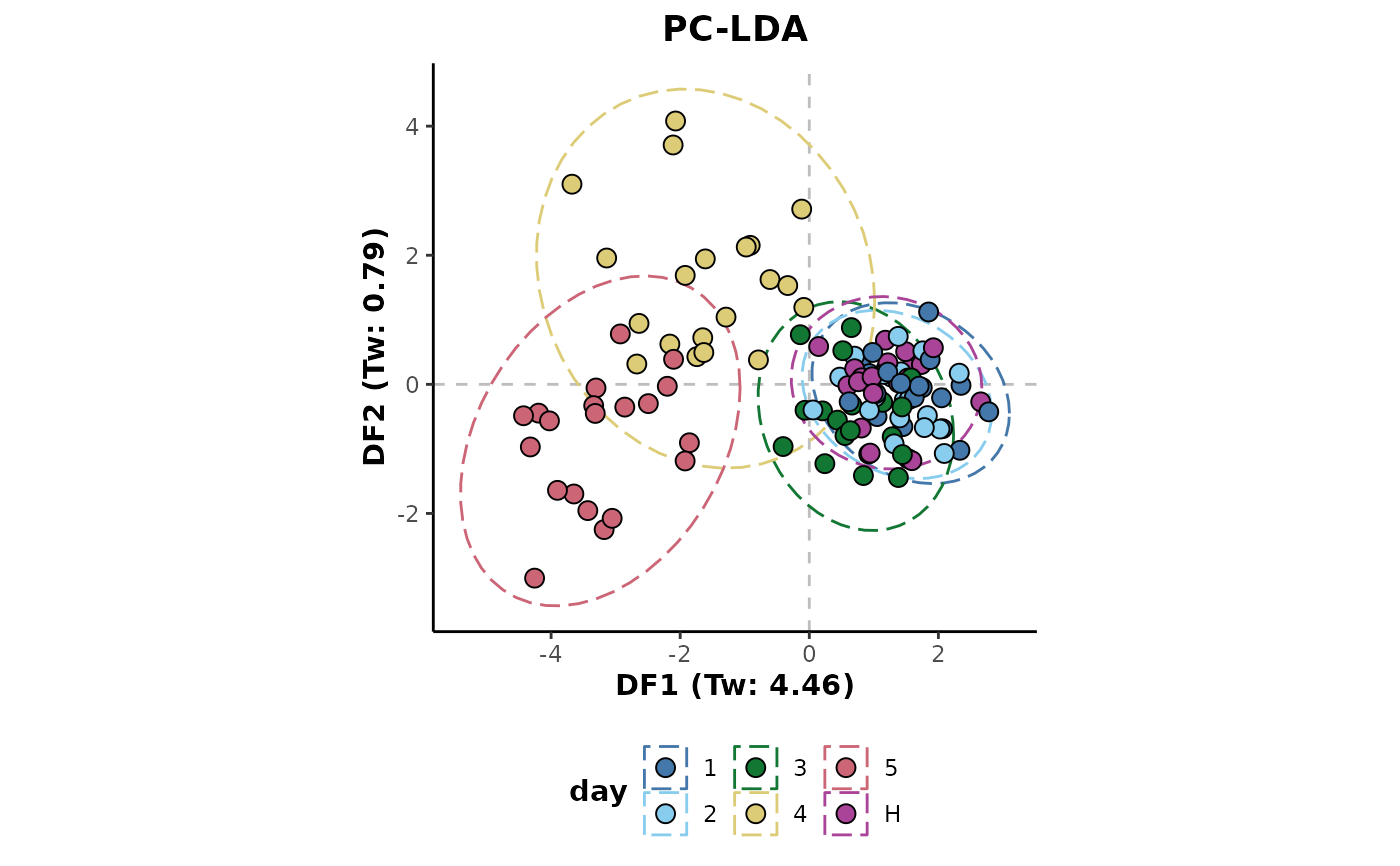
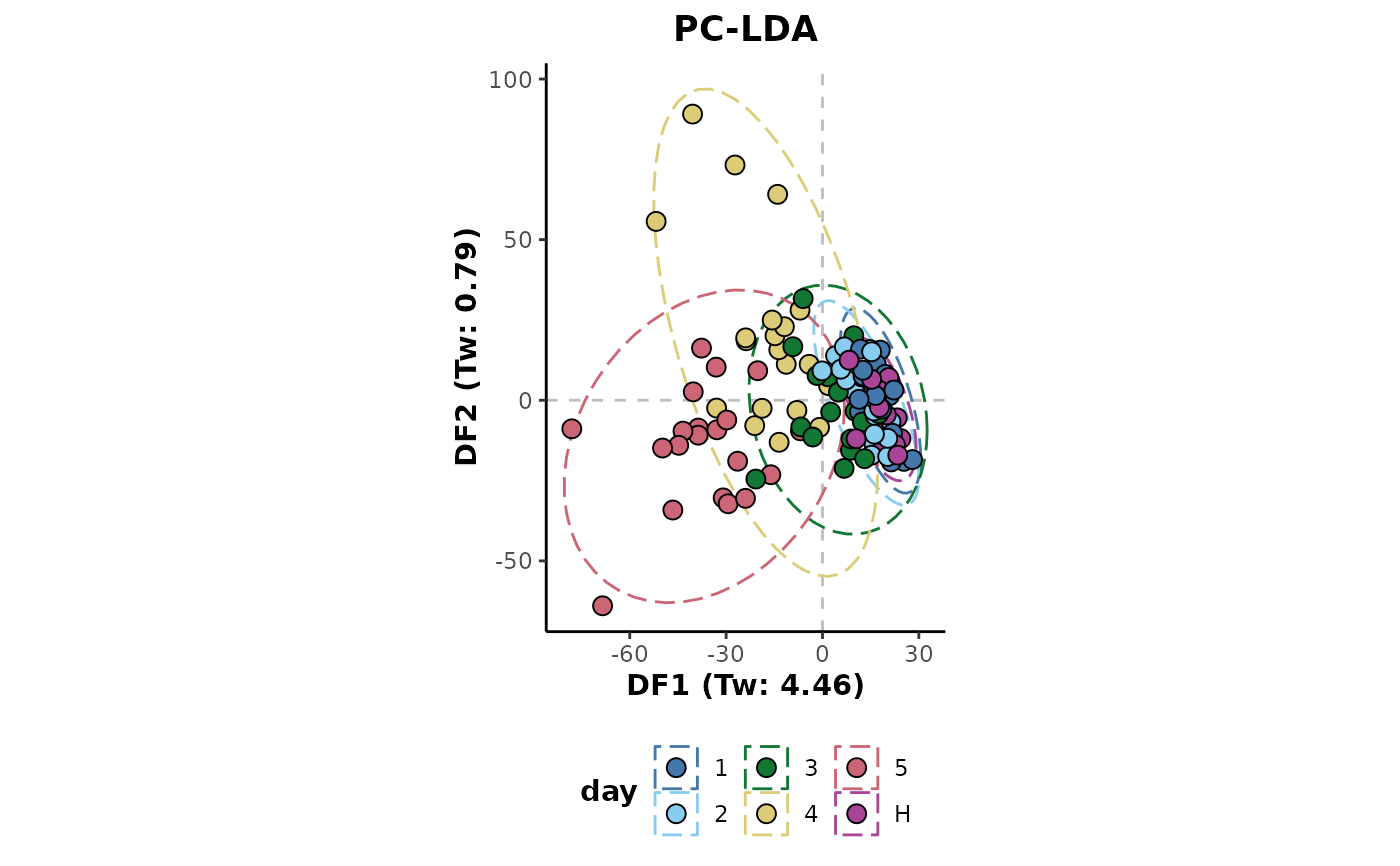
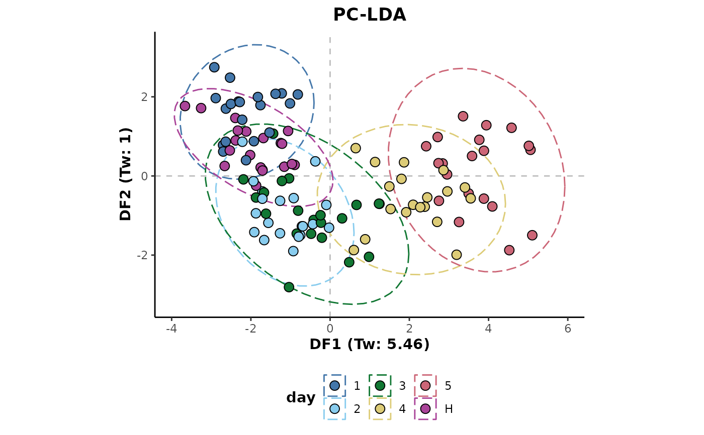
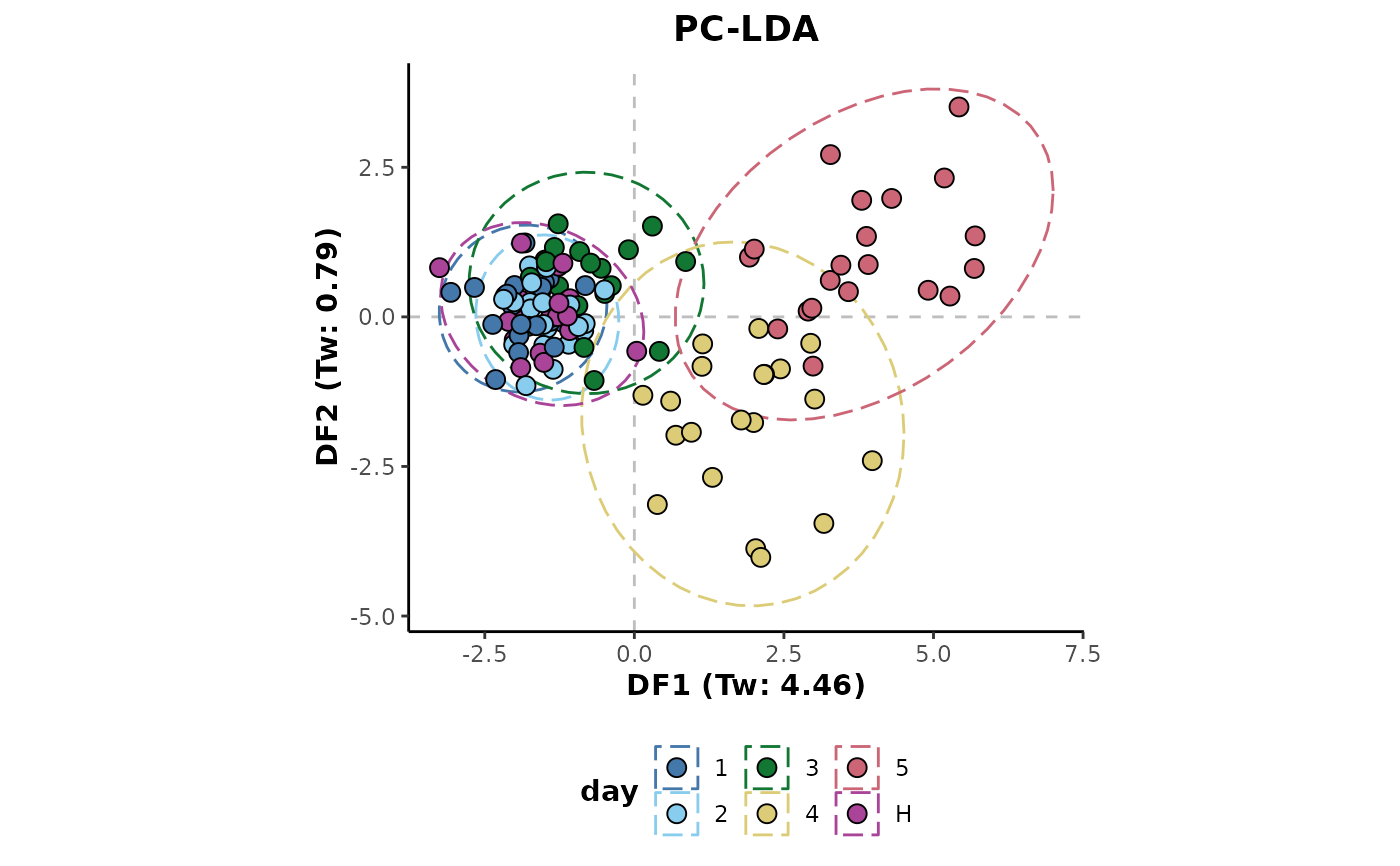
## Each of the following examples shows the application of the transformation and then
## a Linear Discriminant Analysis is plotted to show it's effect on the data structure.
## Initial example data preparation
library(metaboData)
d <- analysisData(abr1$neg[,200:300],abr1$fact) %>%
occupancyMaximum(occupancy = 2/3)
d %>%
plotLDA(cls = 'day')
 ## Arc-sine transformation
d %>%
transformArcSine() %>%
plotLDA(cls = 'day')
 ## Auto scaling
d %>%
transformAuto() %>%
plotLDA(cls = 'day')
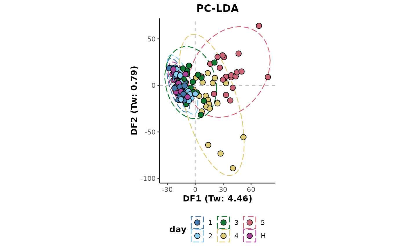
 ## Mean centring
d %>%
transformCenter()%>%
plotLDA(cls = 'day')
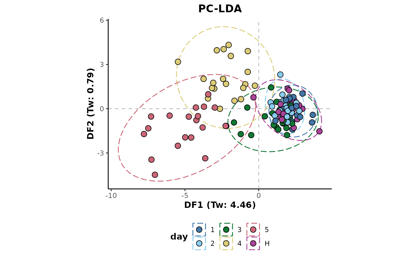
 ## Level scaling
d %>%
transformLevel() %>%
plotLDA(cls = 'day')
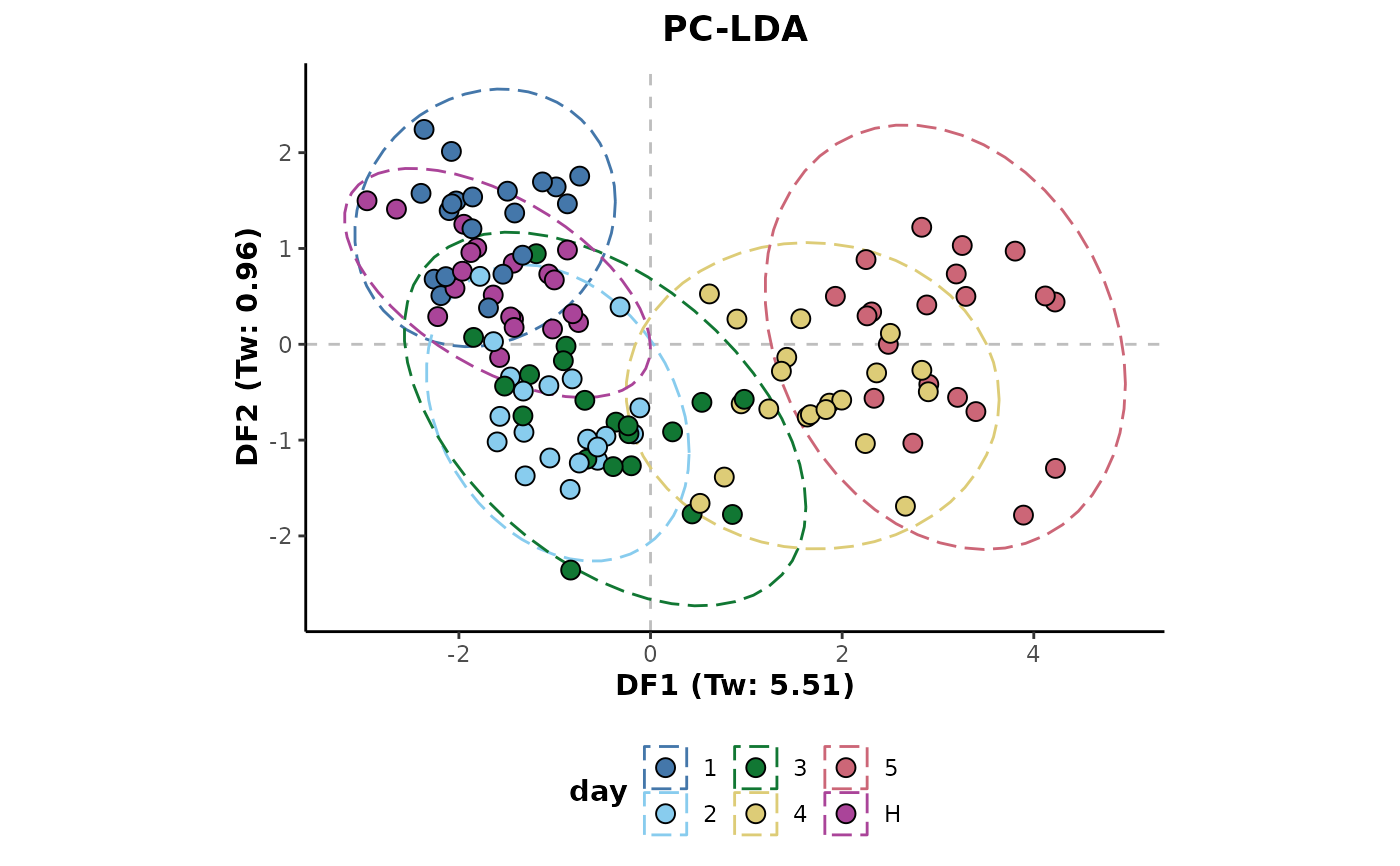
 ## Natural logarithmic transformation
d %>%
transformLn() %>%
plotLDA(cls = 'day')
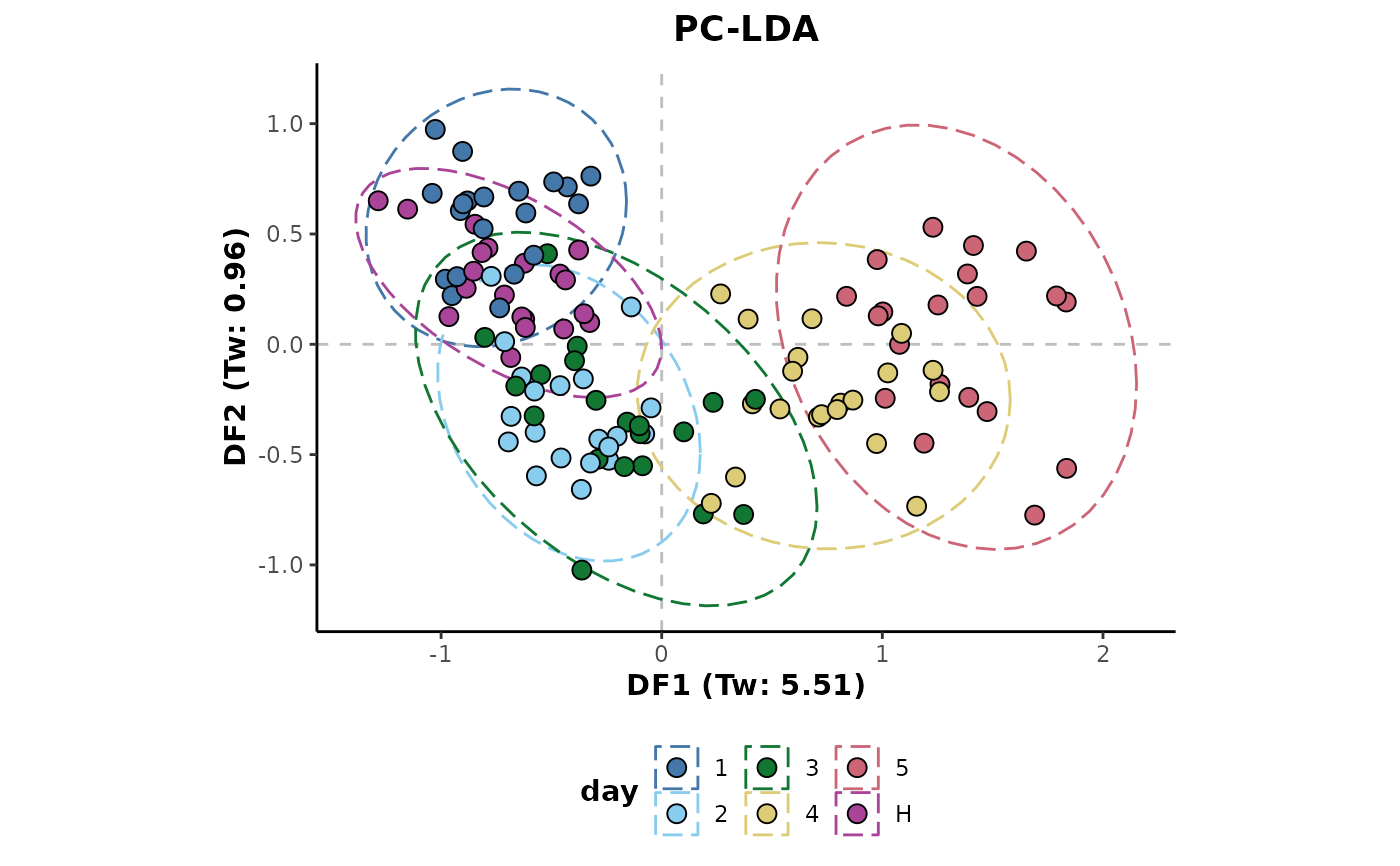
 ## Logarithmic transformation
d %>%
transformLog10()%>%
plotLDA(cls = 'day')
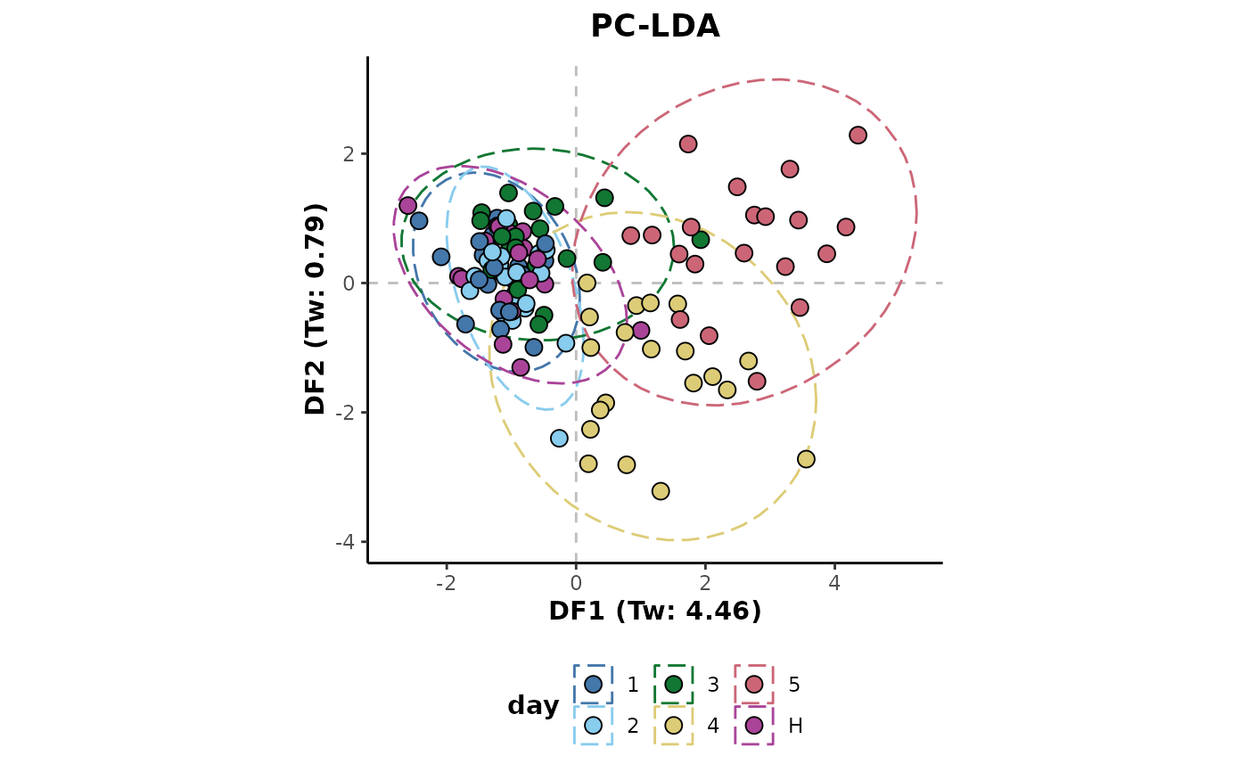
 ## Pareto scaling
d %>%
transformPareto() %>%
plotLDA(cls = 'day')
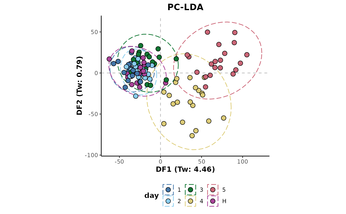
 ## Percentage scaling
d %>%
transformPercent() %>%
plotLDA(cls = 'day')
 ## Range scaling
d %>%
transformRange() %>%
plotLDA(cls = 'day')
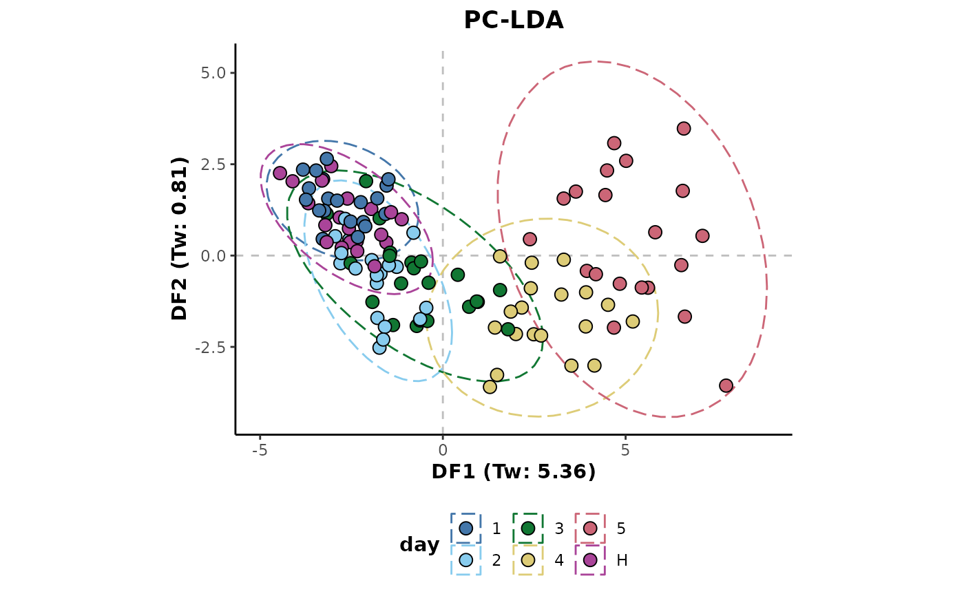
 ## Square root scaling
d %>%
transformSQRT() %>%
plotLDA(cls = 'day')
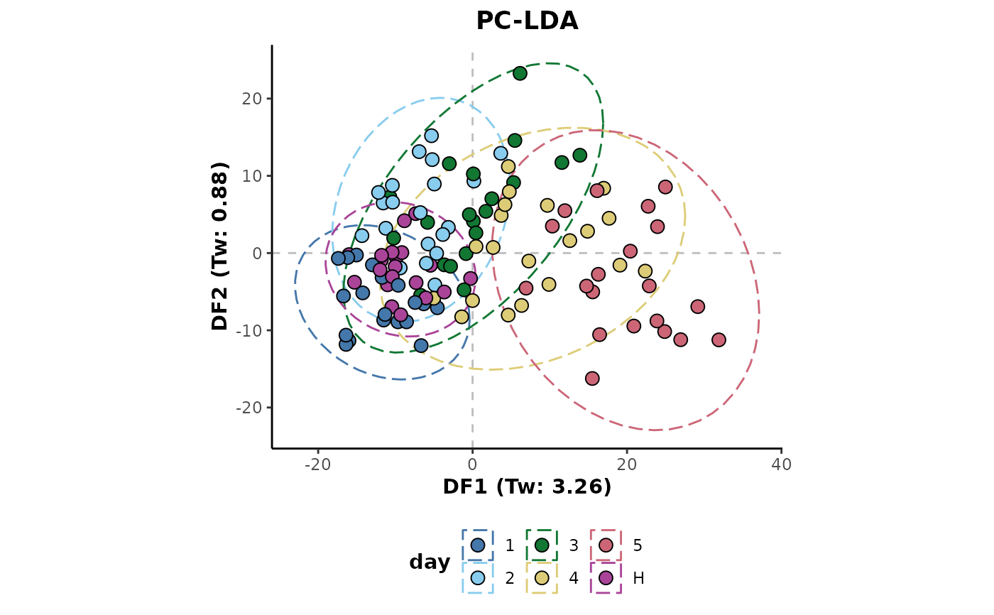
 ## Total ion count nromalisation
d %>%
transformTICnorm() %>%
plotLDA(cls = 'day')
 ## Vast scaling
d %>%
transformVast() %>%
plotLDA(cls = 'day')
